
How much [Beta] is too much?
And the wonders of leverage

I have to warn you up front— there are some actionable takeaways from this piece, but after writing it, I’m left with more unanswered questions than answered ones. The whole catalyst for this post was a comment from a reader asking about how much beta is the right amount of beta—a question that sent me deep down a rabbit hole, that I’ve been thinking on and off about for a number of years.
Before we dive in, if you like my writing please do share it— as I do this for free, the only reward I get from my writing is the feedback from others.
The rabbit hole
If you know nothing about portfolio management, a good place to start is with reading Dalio. Risk parity is a beautiful concept— the combination of uncorrelated risks means that some positions will zig while others zag, resulting is a steadier, lower volatility return stream.
When I moved from being a quant to focusing on fundamental investing, this felt like an obvious foundation to portfolio management. Each position, be it an option, stock, bond, whatever, can act as a differentiated return source in a portfolio. The issue is that each position remains correlated— through duration, beta, or other factors. So once you have your portfolio of positions, the next step is to start managing those cross-position exposures, adding or subtracting factors, beta, and duration until you’re happy with the result.
I still believe position-first is the right order of operations in managing a portfolio, but it immediately begs an obvious questions— what is the right amount of those secondary factors to be taking? How much duration, beta, or value / momentum / growth factor is optimal? And how much is too much of a good thing?
While I believe my methodology here can be replicated for other exposures, for stock pickers beta is by far and away the most important consideration. If beta has a historically positive return, more is better, right? But what are the limitations, and how much is too much? What can we learn from history, and what other factors must be considered?
What history tells us
When people talk about “beta” they’re generally referring to the SP500 index, and exposure to its returns. This is largely due to the liquidity in associated products— be it ETFs, baskets of the underlying components, or futures and options. But the best part about this definition of beta, is that we have an enormous amount of historical data on it.
Shiller has some enormously comprehensive data sets over time, available for free on his website, but even Yahoo Finance and other free sources have daily close and dividend data going back to the 1920’s. And with all these free sources, it’s pretty easy to take daily data from the past c. 95 years and see what happens when you lever the beta over time.
So what is the results?
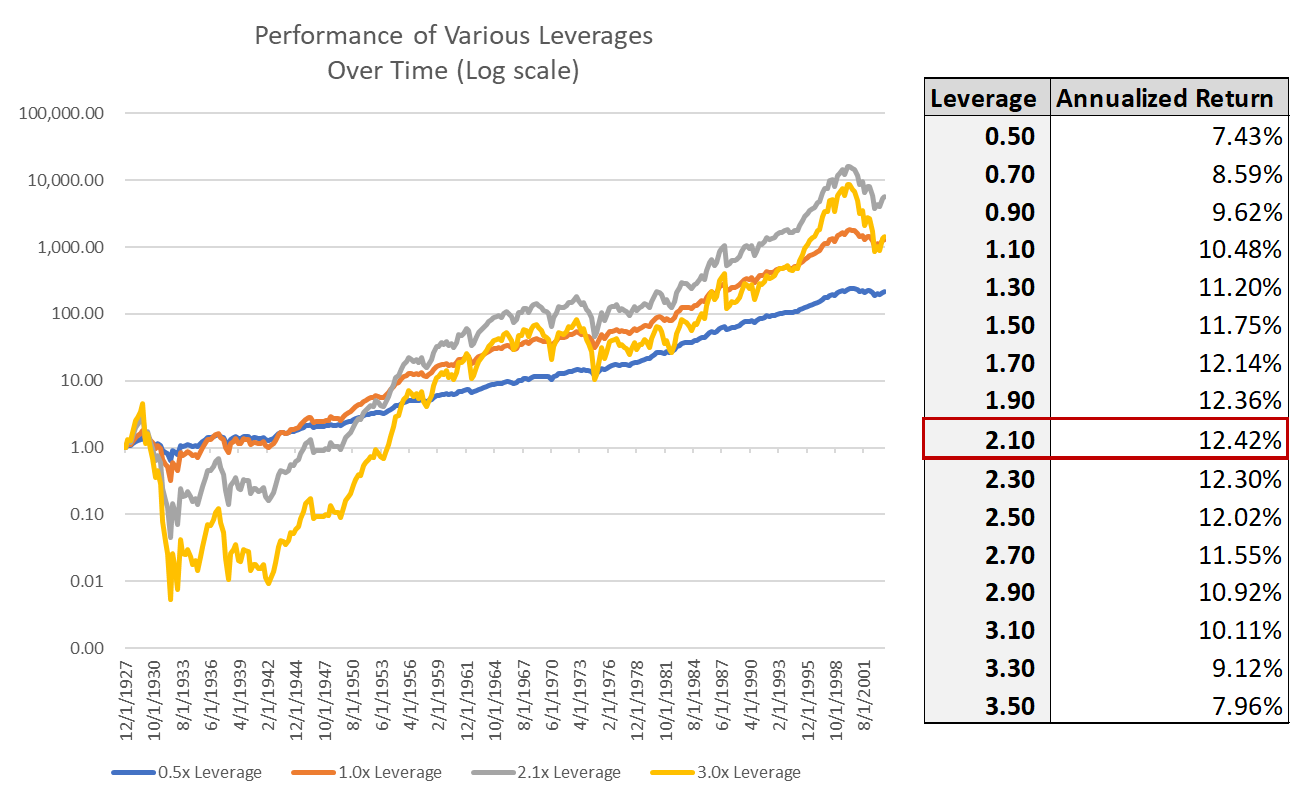
If you take lever the SP500, rebalancing to the given exposure each day, with a borrowing cost at that days short term risk free rate, the optimal amount of leverage is 2.1x. That is the leverage that produces the highest historical return, with the added volatility on any additional leverage dragging returns lower again.
Why does higher Beta cause your returns to decline after 2.1x? Let’s say you have a return that goes down 10% one day, and up 10% the next. While the arithmetic average of this is 0%, the geometric return is -1% (100 → 90 → 99). The difference between the 0% and the 1% scale with the volatility of our returns, for example a +50% / -50% ends with 0% arithmetic / -25% geometric return (100 → 50 → 75). The approximation quants have come up here is the difference is equal to σ^2 / 2.
In other words, while the levered arithmetic return scales linearly, the volatility drag scales exponentially, and at a certain point the additional volatility drag outweighs the additional return from leverage. Adding leverage also adds to your risk of ruin— e.g., 3x leverage on a -35% return will wipe out your entire capital base, not allowing for any incremental returns, and the lifetime return of your portfolio will forever stay at -100%.
Borrowing costs
A couple quick notes on the basic leverage analysis above. First, note that I am only showing out-of-sample performance here1. Second, the above assumes cost of leverage at the 3-month treasury rate over time. This is important to note, as its not the most realistic cost of capital. However, using a moving historical reference is important here. When borrowing costs are higher, the cost of leverage eats into your returns, adding the same amount of volatility drag, but reducing the benefit of leverage. This makes adding more leverage less and less attractive when capital is expensive.
So under different rate environments, what does the optimal leverage look like?
Well right now, margin rates are at c. 6%, implying a reduction in optimal leverage from 2.1x to 1.5x.
Tactical strategies
But let’s take this a step further. There are numerous ideas from systematic finance that can be applied here, but two stand out as easily applicable, well tested, and non-proprietary— vol targeting and trend following.
Vol Targeting
There are two observations regarding volatility that are important to point out. First, volatility is heteroskedastic in regard to return— in simple terms vol is generally highest as markets are crashing. In these periods, the daily swings up and down get crazier, and yet the expected return remains the same. And as volatility is a drag on returns, this pushes both the risk of loss higher, and the expected return lower during these periods. Second, volatility is sticky— the best predictor of future vol is trailing vol.
When you put these two facts together there is an obvious implication— when realized volatility is high, it is best to reduce your exposure. A simple way to do this is scale down exposure by a linear factor of volatility above some hurdle. A backtest of SP500 returns levered at the lesser of 2.1x or [(15%) / (historical vol)] * (2.1) shows this strategy outperforms a basic 2.1x leverage— largely due to the outperformance during the great depression:
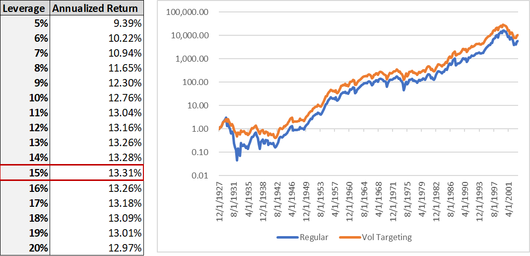
I would caution, however, that given the outperformance of this strategy is largely based around a single event, this result does seem somewhat overoptimized to me— and I would use caution in implementing such a strategy on a go forward basis. That said, vol targeting has been proven to be fairly robust across other quant strategies
Trend Following
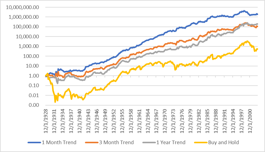
The second lesson from quantitative finance is that across almost all tested time frames, and across numerous assets, things “going up” continue “going up”. Beta is no exception here. A simple back test shows that a trend following strategy2 vastly outperforms a buy and hold strategy.
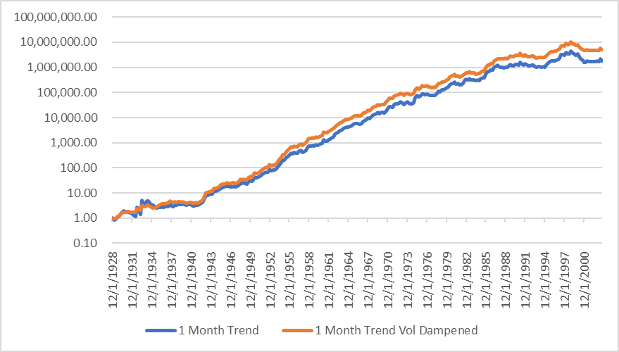
And here’s a bonus third lesson from the systematic world; combining diversifying strategies is usually better than any single strategy alone. A vol-capped trend following strategy should combine the benefits of both risk reduction and momentum to create a return stream that is even better than what we had tested separately. And looking at our back test, a combined strategy works well.
So what does history tell us to do in some? It tells us we should:
Have a portfolio’s beta defined by a trend following strategy (here I use 1-month SMA, +2.5x when long -0.5x when short)
Cap volatility at 15%
Probably time for a disclaimer: NONE OF THIS IS INVESTMENT ADVICE. I also think there are legitimate issues with this strategy (including the rate sensitivity described above, etc.), and the exact numbers are significantly overoptimized in an out-of-sample regression.
What history can’t teach us
Past performance is no guarantee of future results.
Back tests are great, but they create a number of problems. First and foremost, they create overfitting. The more parameters a strategy has in its back test, the less likely it will perform well during live trading. This is why all systematic strategies must be created on out of sample data, and then re-tested in sample to ensure we’re not just extrapolating from a historical anomalies. While trend following and volatility dampening have been well proven across time and markets, it doesn’t mean that the exact parameters can’t be over optimized. Whether it be target vol, the length of a SMA in trend following, or— most importantly— the target leverage, there is no guarantee past results are predictors of future performance.
Another reason for this is that while to an investor staring at index returns, the markets look like a random walk, in reality price movements are the culmination of hundreds of thousands of investors making decisions every day. The decision these investors make, and the way they make them (e.g., the market microstructure) change over time. There is no reason to believe that the SP500 of the next 100 years should perform the way it did in the past century. That isn’t to say it will perform worse, just that there is no way of knowing.
Rules of Thumb
While the back tests may indicate you should be levering more than we anticipated, there are a couple heuristics and pragmatic limitations that may say otherwise, and largely have to do with drawdowns.
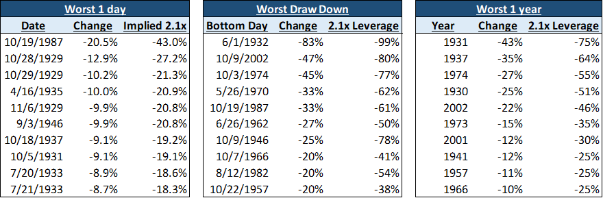
The worst one day draw down in SP500 history was the famous Black Monday. This shows the obvious limits of leverage— at 5.0x leverage a single day draw down would have wiped out a portfolio. But even 2.0x or 3.0x leverage creates enormous one day drawdowns. And who is to say that there isn’t a greater drawdown at some point in the future? If we’ve seen markets drop 20% in a day, why can’t they drop 30% or more?
The overall draw downs expand on this even more— the 2002 draw down would have been 80% for a “properly” levered fund. What is a fund managers ability to come back from losses like that? The reality of asset management starts to kick in— what is the managers ability to continue levering the fund cross cycles at that level? That ignores the fact that LPs would pull their dollars back with even a small part of that drawdown. But even if they didn’t, with a high water mark the manager wouldn’t be able to charge incentive fees until they made a subsequent 500% return— their ability to keep talent would be next to zero.
The other reality here is that managers are largely measured on their return per unit of risk, not the long term compounded growth rate of their investments. So optimizing for maximum long term return is really not the equation most asset managers make.
Is the SP500 special?
The other issue here is broader— since 1927, the SP500 has outperformed almost all international markets. Why should this continue on a go forward basis? This specific analysis ends shortly after the dot-com bubble, a historically unprecedented run-up in stocks.
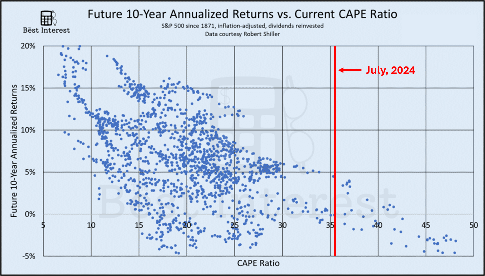
Today, market valuations aren’t as high as they were during the dotcom bubble, but based on historical regression vs. the CAPE ratio, they are certainly pointing to flat to single digit go-forward real returns. Should that mean the go-forward optimal solution is the same is the past? I’m not sure, but leveraging your portfolio is an explicit bet that you think the equity return will be higher than rates, and with margin rates at 6%, that’s a fairly high hurdle.
It’s worth noting that while executing this analysis I did look at back tests on using market valuations as another variable and it doesn’t create an outperformance— the timeline is too long. But there is still an overarching implication the go forward performance will be different than the last 100 years combined.
Conclusion
This work has raised more questions than answers for me. Historical analysis indicates you should take more leverage than you might believe at first. But heuristics of go future performance say you should be careful. The whole analysis is sensitive to rates and rates are high right now. Active strategies are great, but peter out on the back end of the out-of-sample data.
I was discussing with my old PM and he also made an interesting point, which is the CFOs of each SP500 constituent (who arguably should have the best information) is making the decisions about how to “optimally” lever the company. On an aggregate, the market already includes the asset level leverage, and therefore the aggregate level of beta may be fairly close to 1.0x— implicitly trusting the underlying asset leverage.
Similar to Kelly, I think the answer is you want to be inside of “optimal” to create some margin of safety, but the market likely does underestimate the power of leverage to increase long term returns.
This is also only a discussion on margin leverage— what about other forms of fixed borrowing costs? What if you can find alternative forms of leverage (e.g., shorting, insurance float, securitization, NAV loans etc.) that can increase your leverage without the variability. I guess I’ll have to leave that for another post.
If you enjoyed this, I would kindly as you share and subscribe. The more my work is widely shared, the more I’ll be incentivized to find the time to keep writing.
I’ve been using in-sample to confirm my hypothesis for very specific strategies, and therefore don’t have in-sample productions of many of these more broad tests. That said, the data is easily available to replicate my findings for the past 20-years.
Here I am using simple SMA cross over strategies— e.g., when the previous daily close is higher than the trailing simple moving average that is a signal to buy, and when it is not, that is a signal to sell. All strategies shown are long 2.5x beta when a buy signal is ongoing, the one month is short 0.5x beta while the other two take no position while a sell signal is ongoing.